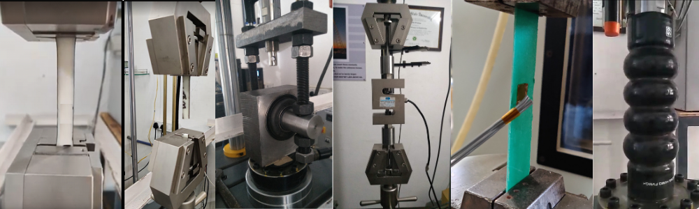
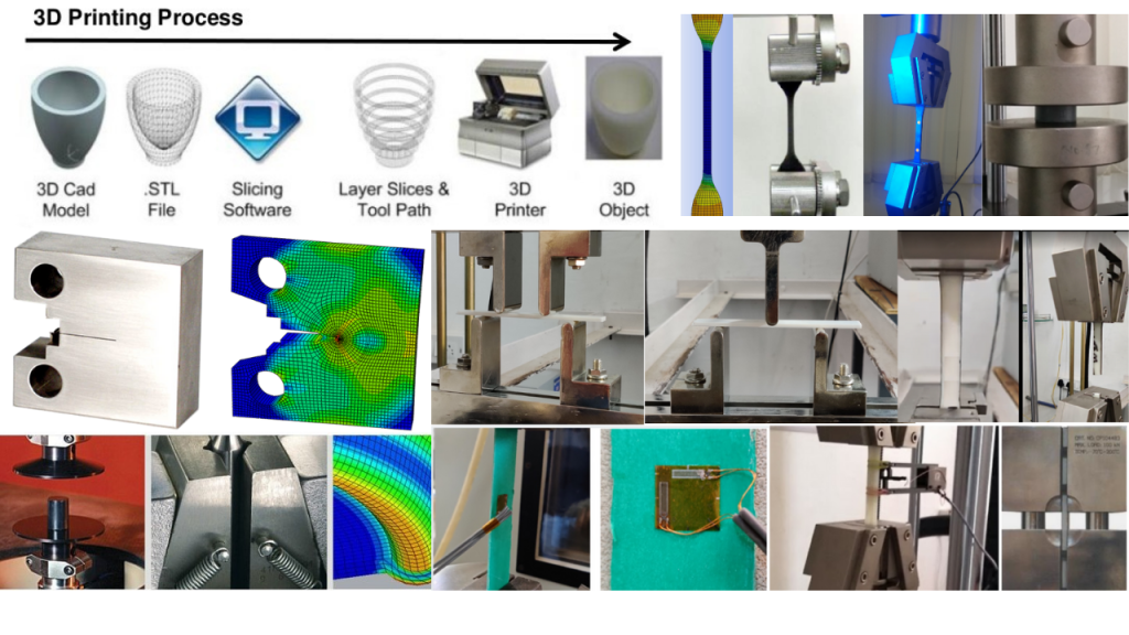
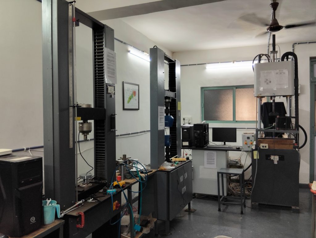
Every test we conduct at our laboratory is a real-world engineering problem. A rubber component, metal structure, polymer part, or composite assembly arrives with a failure, a performance target, or an unanswered question. The specimen has to be prepared correctly, gripped without inducing artifacts, instrumented precisely, tested under controlled conditions, and interpreted with engineering judgment grounded in mechanics and material behavior. Get any one of those wrong, and the data loses meaning.
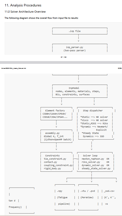
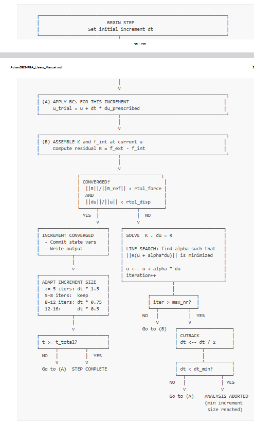
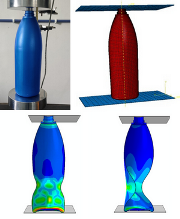
Our FEA and durability engineering work adds another layer of complexity. A FEA simulation is only as good as the assumptions behind it. Material models have to capture real-world nonlinear behavior. Boundary conditions must represent operating reality, not idealized textbook cases. Fatigue life predictions depend on how accurately strain energy, contact mechanics, crack initiation, and load histories are understood. We routinely work on problems where a few millimeters of displacement, a small stress concentration, or a slight variation in material behavior can determine whether a component survives millions of cycles or fails prematurely in the field.
Engineering in the physical world rarely behaves perfectly. Machines drift out of calibration. Samples vary from batch to batch. Real loading conditions are seldom clean or repeatable. Components see heat, vibration, dirt, overloads, misuse, and manufacturing variations that no specification sheet fully captures. And beyond the technical complexity, we build and operate in India – where industries move at different levels of maturity, testing standards are interpreted differently across sectors, documentation can be incomplete, and engineering decisions are often made under severe cost and time pressures. This is not a limitation; it is the environment that shapes our capability. Because building reliable engineering systems in these conditions requires more than software or machinery. It requires experience, discipline, experimentation, and the ability to bridge theory with manufacturing reality. Over the years, we have built a practice that does not depend on ideal assumptions. Our strength lies in understanding how products behave in actual service conditions and helping customers make engineering decisions with confidence.
As a result, our laboratory and engineering services have become trusted partners for manufacturers, OEMs, suppliers, and product development teams across industries.
Our work supports the development and validation of components that operate in demanding environments – from automotive and industrial systems to rubber and polymer applications where durability and reliability are critical. Every project we complete strengthens not only the products we help validate, but also the engineering ecosystem that depends on accurate testing, dependable analysis, and practical problem-solving.
For more information, contact us