Plastics are ubiquitous in our daily lives, used in a wide range of applications due to their versatility, durability, and cost-effectiveness. However, when exposed to elevated temperatures, some plastics may deform or lose their structural integrity, compromising their functionality and safety. This is where heat deflection testing plays a crucial role in assessing a plastic material’s ability to withstand heat and maintain its shape under load. In this blog post, we will delve into the importance of heat deflection testing for plastics and explore its significance in ensuring material reliability and performance.
Are you curious about the performance of plastics under high temperatures? Discover the significance of heat deflection testing for plastics, ensuring their reliability and performance in various applications.
Understanding Heat Deflection Testing:
Heat deflection testing, also known as heat distortion testing or HDT, is a standardized method used to evaluate a plastic material’s ability to resist deformation under load at elevated temperatures. It determines the heat deflection temperature (HDT) or the temperature at which a specific deformation or deflection occurs in the plastic specimen. This testing method helps manufacturers and engineers select the most suitable plastic materials for applications involving high temperatures.
AdvanSES VST HDT Apparatus
Importance of Heat Deflection Testing:
2.1. Ensuring Material Reliability:
Heat deflection testing provides vital insights into a plastic material’s ability to maintain its structural integrity when exposed to elevated temperatures. By subjecting plastics to controlled heating and measuring their deformation under load, manufacturers can identify materials that can withstand the intended operating conditions without significant deformation or failure. This ensures that the final products will perform reliably and maintain their shape, avoiding costly failures or safety hazards.
2.2. Performance Optimization:
Different plastics exhibit varying thermal properties, including their response to temperature changes. Heat deflection testing helps engineers optimize material selection for specific applications where exposure to heat is a concern. By comparing HDT values of different plastics, manufacturers can choose materials with higher HDT values that can withstand higher temperatures, resulting in improved product performance and longevity.
Conducting Heat Deflection Testing:
3.1. Standards and Test Methods:
Heat deflection testing follows established standards such as ASTM D648 (Standard Test Method for Deflection Temperature of Plastics Under Flexural Load in the Edgewise Position) and ISO 75 (Plastics—Determination of Temperature of Deflection Under Load). These standards provide specific guidelines for test specimen preparation, loading conditions, and temperature ramp rates, ensuring consistent and comparable results across different laboratories.
3.2. Test Equipment:
Heat deflection testing requires specialized equipment, typically including a testing machine capable of applying a load on the plastic specimen and a heating chamber or furnace to control the temperature. The test machine measures the deflection of the specimen while it is subjected to a specified load at increasing temperatures until a predefined deflection value is reached.
Applications of Heat Deflection Testing:
Heat deflection testing is essential in numerous industries where plastics are used in high-temperature environments. Some key applications include automotive components, electrical enclosures, consumer electronics, aerospace parts, and industrial equipment. By subjecting plastic materials to rigorous heat deflection testing, manufacturers can ensure the long-term performance and reliability of their products.
Conclusion:
Heat deflection testing is a vital aspect of evaluating plastics’ performance and reliability when exposed to high temperatures. By conducting this testing, manufacturers and engineers can select appropriate materials for specific applications, optimize product performance, and minimize the risk of deformation or failure. Ultimately, heat deflection testing contributes to the overall quality, safety, and longevity of plastic-based products in various industries.
Looking to optimize plastic materials’ performance in high-temperature environments? Contact our experts today to learn how heat deflection testing can enhance the reliability and longevity of your products.
A proper treatment of the rubber material testing service conditions and material degradation phenomena like strain softening is of prime importance in the testing of rubbers specimens for FEA material characterization. The accuracy and reliability of obtained test data depends on how the mechanical conditioning and representational service conditions of the material have been accounted for in the test data. To simulate a component in unused and unaged conditions, the mechanical conditioning requirements are different than the ones for simulating a component that has gone through extensive field service and aging under different environmental conditions.
To simulate performance of a material or component by Finite Element Analysis (FEA) it should be tested under the same deformation modes to which original assembly will be subjected. The uniaxial tension tests are easy to perform and are fairly well understood but if the component assembly experiences complex multiaxial stress states then it becomes imperative to test in other deformation modes. Planar (pure shear), biaxial and volumetric (hydrostatic) tests need to be performed along with uniaxial tension test to incorporate the effects of multiaxial stress states in the FEA model.
Material stiffness degradation phenomena like Mullin’s effect at high strains and Payne’s effect at low strains significantly affect the stiffness properties of rubbers. After the first cycle of applied strain and recovery the material softens, upon subsequent stretching the stiffness is lower for the same applied strain.
Despite all the history in testing hyperelastic and viscoelastic materials, there is a lack of a methodical and standard testing protocol for pre-conditioning. Comprehensive studies on the influence of pre-conditioning are not available. Readers are referred to Austrell[] and Remache, et al,[]. There are no guidelines for sample pre-conditioning in ASTM D412. However, British Standard BS 903 suggests to perform 5 cycles of pre-conditioning to improve test reproducibility.
There are five (5) different techniques to carry out pre-conditioning and material testing of general elastomer samples.
1. The first technique pertains to a mechanical test where the the testing of the sample is carried out under one single stretch at a speed recommended by the ASTM D412 specification.
2. In the second testing technique the sample is stretched at a constant speed up to the maximum relevant strain brought back to the initial position. Cyclic stretching is then carried out for anywhere for 1 to 7 cycles. The speed of the initial stretch and the number of subsequent cyclic stretches needs to be same. The data curve is then shifted to the origin by zeroing out the stress and strain and used for curve-fitting procedure.
3. In the third testing protocol the sample is stretched to a fraction of the full material stretch capability and brought back to the initial position and cycled back again to this fractional position anywhere from 2 to 7 cycles. The stretch in the sample is then increased to the second level and cycled back to initial position multiple times. The sample is stretched back to an even higher position and cycled back. This progressively continues until the maximum strain capability of the material is reached. This protocol is known as progressive pre-conditioning.
4. In the fourth testing technique the sample is stretched to a fraction of the total stretch capability and relaxed for anywhere from 30 seconds to 120 seconds as per the material. The sample is then again stretched to a higher limit and relaxed again. This is continued until the maximum stretchable capability of the material. This particular technique stretches the material and allows the material to fully creep and relax at each interval so that all the stress softening is accounted for in the test data.
5. In the fifth testing technique the sample is tested under a single stretch but the speed or the rate of stretch is very slow. This ultra-slow speed test is carried out so that the material can creep, relax, and the cross-links in the elastomer are given enough time to expand-contract and come to a balanced position during the stretching. This technique is a combination of the two above testing techniques.
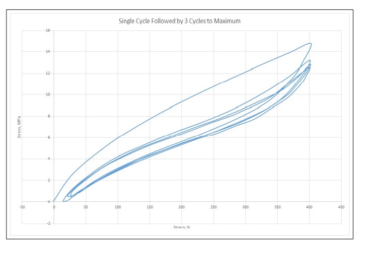
These five (5) testing protocols involve the stretching of the material to different limits under different conditions and suitably cycling the material. The suitability of one testing technique over the other is debatable and one should adopt the technique that most closely resembles the operating conditions of the material and what one expects to back out from the Finite Element Analysis. Figures (1.11) through (1.14) shows the results from using the different testing protocols on a 55 durometer Natural Rubber Compound that finds general application in an automotive engine mount.
Figure 1.11: Uniaxial Tension Test Results
Figure 1.12: Single Stretch Followed by 3 Cycles of Stretching to the Maximum
Figure (1.12) shows the results from comparisons carried out on a uniaxial compression test for an engine mount material characterization. Two protocols were employed to carry out the material characterization. Progressive straining and cycling was carried out first. The material was strained 3 times before reaching the ultimate strain of approximately 75 %. The material was subsequently tested using ultra slow straining protocol. As can be seen the test data output for FEA input is the same using both the techniques. This result confirms the observation by Austrell in his work on conditioning of material samples for characterization i.e., Mullins effect can be negated when enough time is allowed for the material to relax, creep, and flow during the rubber material testing.
Figure 1.13: Progressive Pre-conditioning with Stretching to 3 levels and Cyclic Stretches
Figure 1.14: Progressive Relaxation, Stretching and Relaxation to Maximum Levels
1.2 Guidelines for Rubber Material Testing
Rubber compounds are formulated from recipes of ingredient materials. Depending on the time, location and environment while mixing the compounds, properties are known to vary from batch to batch.
• All testing to characterize a material compound should be performed on the same batch.
• Laboratory validations will help to correlate test specimen slabs against the real components to make sure they have identical cure history.
• Small compression buttons can be extracted from components and compared with slab data.
• The testing should be carried out at the temperature at which the component is expected to perform under field service conditions.
• For seals and o-rings, aging in oils and solutions can be carried out prior to testing.
• Input of more than one test data type in FEA software will increase simulation accuracy by an order of magnitude
AdvanSES announces that its Testing Laboratory has attained ISO/IEC 17025:2017 accreditation vide NABL certificate No. TC-9168. ISO/IEC 17025:2017 is the highest recognized quality standard in the world for calibration and testing laboratories. Accreditation means the lab consistently produces precise and accurate test data and has implemented a rigorous quality management system. The stringent processes in the audits for the accreditation relate to the operations, efficiency and effectiveness of the laboratory. Test data from the laboratory is benchmarked for accuracy, reliability and consistency.
Receiving the accreditation means that test reports and certificates generated from AdvanSES laboratory can now be generally accepted from one country to another without further testing.
The scope of the accreditation covers tests and properties in the field of rubbers, plastics and composite materials. It is one of the few labs in the world accredited to perform internationally recognized fatigue standards like ASTM D7791.
AdvanSES today is one of the few companies in the world who provide expert problem solving services using Finite element analysis (FEA), provides new product development and material testing and analysis.
The finite element method (FEM) is a numerical method
used to solve a mathematical model of a given structure or system, which are
very complex and for which analytical solution techniques are generally not
possible, the solution can be found using the finite
element method. The finite element
method can thus be said to be a variational formulation method using the principle of minimum potential
energy where the unknown quantities of interests are approximated by continuous piecewise polynomial functions. These quantities
of interest can be different according to the chosen system, as the finite
element method can be and is used in various
different fields such as structural mechanics, fluid mechanics, accoustics, electromagnetics,
etc. In the field of structural mechanics the primary field of interest is the
displacements and stresses in the system.
It is important to understand that FEM only gives an approximate solution of the prob- lem and is a numerical approach to get the real result of the variational formulation of partial differential equations. A finite element based numerical approach gives itself to a number of assumptions and uncertainties related to domain discretizations, mathematical shape functions, solution procedures, etc. The widespread use of FEM as a primary tool has led to a product engineering lifecycle where each step from ideation, design development, to product optimization is done virtually and in some cases to the absence of even prototype testing.
This fully virtual product development and analysis methodology leads to a situation where a misinterpreted approximation or error in applying a load condition may be car- ried out through out the engineering lifecycle leading to a situation where the errors get cumulative at each stage leading to disastrous results. Errors and uncertainties in the ap- plication of finite element method (FEM) can come from the following main sources, 1) Errors that come from the inherent assumptions in the Finite element theory and 2) Errors and uncertainties that get built into the system when the physics we are seeking to model get transferred to the computational model. A common list of these kind of errors and uncertainties are as mentioned below;
Errors and uncertainties from the solver.
Level of mesh refinement and the choice of element type.
Averaging and calculation of stresses and strains from the primary solution variables.
Uncertainty in recreating the geometrical domain on a computer.
Approximations and uncertainties in the loading and boundary conditions of the model.
Errors coming from chosing the right solver types for problems, e.g. Solvers for eigen value problems.
The long list of error sources and uncertainties in the procedure makes it desirable that a framework of rules and criteria are developed by the application of which we can make sure that the finite element method performs within the required parameters of accuracy, reliability and repeatability. These framework of rules serve as verification and validation procedures by which we can consistently gauge the accuracy of our models, and sources of errors and uncertainties be clearly identified and progressively improved to achieve greater accuracy in the solutions. Verifications and Validations are required in each and every development and problem solving FEA project to provide the confidence that the compu- tational model developed performs within the required parameters. The solutions provided by the model are sufficiently accurate and the model solves the intended problem it was developed for.
Verification procedure includes checking the design, the software code and also investigate if the computational model accurately represents the physical system. Validation is more of a dynamic procedure and determines if the computational simulation agrees with the physical phenomenon, it examines the difference between the numerical simulation and the experimental results. Verification provides information whether the computational model is solved correctly and accurately, while validation provides evidence regarding the extent to which the mathematical model accurately correlates to experimental tests.
In addition to complicated
discretization functions, partial differential equations repre- senting physical systema, CFD and FEA both use
complicated matrices and PDE solution algorithms to solve physical systems.
This makes it imperative to carry out verification and validation activities
separately and incrementally during the model building to ensure reliable processes. In order to
avoid spurious results and data contamination giving out false signals, it is
important that the verification process is carried out before the valida- tion
assessment. If the verification process fails the the model building process
should be discontinued further until the verification is established. If the
verification process suc- ceeds, the
validation process can be carried further for comparison with field service and
experimental tests.
1.2 Brief History of Standards and Guidelines for Verifi- cations and Validations
Finite element analysis found widespread use with the release of NASA Structural Anal- ysis Code in its various versions and flavous. The early adopters for FEA came from the aerospace and nuclear engineering background. The first guidelines for verification and validation were issued by the American Nuclear Society in 1987 as Guidelines for the Ver- ification and Validation of Scientific and Engineering Computer Programs for the NuclearIndustry.
The first book on the subject was written by Dr. Patrick Roache in 1998 titled Verification and Validation in Computational Science and Engineering, an update of the book appeared in 2009.
In 1998 the Computational Fluid Dynamics Committee on
Standards at the American Institute of Aeronautics and Astronautics released
the first standards document Guide for
the Verification and Validation of Computational Fluid Dynamics Simulations.
The US Depeartment of Defense through Defense Modeling and Simulation Office
releaseed the DoD Modeling and
Simulation, Verification, Validation, and Accreditation Document in 2003.
The American Society of Mechanical Engineers (ASME) V
and V Standards Commit- tee released
the Guide for Verification and Validation in
Computational Solid Mechanics (ASME V and V-10-2006).
In 2008 the National Aeronautics and
Space Administration Standard for Models
and Simulations for the first time developed a set of guidelines that provided a numerical score for
verification and validation efforts.
American Society of Mechanical Engineers
V and V Standards Committee
V and V-20 in 2016 provided
an updated Standard for Verification and Validation in Computational Fluid Dynamics and Heat Transfer .
1.3 Verifications and Validations :- Process and Procedures
Figure(1.1)
shows a typical product design cycle in a fast-paced industrial product de- velopment group. The product interacts
with the environment in terms of applied loads,
boundary conditions and ambient atmosphere. These factors form the
inputs into the com- putational model
building process. The computational model provides us with predictions and
solutions of what would happen to the product under different service conditions.
It
is important to note that going from the physical
world to generating a computational model
involves an iterative process where
all the assumptions, approximations and their effects on the the quality of the computational model are iterated
upon to generate the most optimum
computational model for representing the physical world.
Figure 1.1: Variation on the Sargent Circle Showing the Verification and Validation Procedures in a Typical Fast Paced Design Group
The validation process between the
computational model and the physical world also involves an iterative process,
where experiments with values of loads and boundary con- ditions are solved and
the solution is compared to output from the physical world. The computational
model is refined based upon the feedbacks obtained during the procedure.
The circular shapes of the process
representation emphasizes that computational mod- eling and in particular
verification and validation procedures are iterative in nature and require a
continual effort to optimize them.
The blue, red and green colored
areas in Figure(1.3)
highlight the iterative validation and
verification activities in the process. The standards and industrial guidelines
clearly mention the distinctive nature of code and solution
verifications and validations at different levels.
The green highlighted region falls in the domain of the laboratory performing
the experiments, it is equally important
that the testing
laboratory understands both the process and procedure of verification and
validation perfectly.
Code verification seeks to ensure
that there are no programming mistakes or bugs and that the software
provides the accuracy
in terms of the implementation of the numerical al- gorithms or construction of the solver. Comparing
the issue of code verification and calcu- lation verification of softwares, the main point of difference is that calculation verification
Figure 1.2: Verification and Validation Process
involves quantifying the discretization error in a numerical simulation. Code verification is rather upstream in the process and is
done by comparing numerical results with analytical solutions.
Figure 1.3: Guidance for Verification and Validation as per ASME 10.1
Standard
1.4 Guidelines for Verifications and Validations
The first step is the verification of the code or software
to confirm that the software
is work- ing as it was
intended to do. The idea behind code verification is to identify and remove any
bugs that might have been generated
while implementing the numerical algorithms or
because of any programming errors. Code verification is primarily a
responsibility of the code developer and softwares like Abaqus, LS-Dyna
etc., provide example
problems man- uals, benchmark manuals to show the
verifications of the procedures and algorithms they have implemented.
Next step of calculation verification
is carried out to quantify the error in a computer simulation due to factors
like mesh discretization, improper convergence criteria, approxi- mation in material
properties and model generations. Calculation verification provides with an
estimation of the error in the solution because of the mentioned factors.
Experience has shown us that insufficient mesh discretization is the primary
culprit and largest
contributor to errors in calculation verification.
Validation processes for material models, elements, and numerical algorithms are gen- erally part of FEA and CFD software help manuals. However, when it comes to establishing the validity of the computational model that one is seeking to solve, the validation procedure has to be developed by the analyst or the engineering group.
The
following validation guidelines were developed at Sandia National
Labs[Oberkampf et al.] by experimentalists working on wind tunnel
programs, however these are
applicable to all problems from computational
mechanics.
Guideline 1: The validation experiment
should be jointly designed by the FEA group and the experimental engineers. The
experiments should ideally be designed so that the validation domain falls
inside the application domain.
Guideline 2: The designed experiment
should involve the full physics of the system, including the loading and
boundary conditions.
Guideline 3: The solutions of the
experiments and from the computational model should be totally independent of each other.
Guideline 4: The experiments and the validation process should start from the system level solution to the component level.
Guideline 5: Care should be taken that operator bias or process bias does not
contami- nate the solution or the validation process.
1.5 Verification & Validation in FEA
1.5.1 Verification Process of an FEA Model
In the case of automotive product development problems, verification of components like silent blocks and bushings, torque rod bushes, spherical bearings etc., can be carried. Fig- ure(1.4) shows the rubber-metal bonded component for which calculations have been carried out. Hill[11], Horton[12] and have shown that under radial loads the stiffness of the bushing can be given by,
Figure 1.4: Geometry Dimensions of the
Silent Bushing
converted PNM file
Figure 1.5: Geometry of the Silent Bushing
and G= Shear Modulus = 0.117e0.034xHs, Hs = Hardness of the material. Replacing the geometrical values
from Figure(1.4),
Krs= 8170.23N/mm, (1.3)
for a 55 durometer
natural rubber compound. The finite element model for the bushing
is shown in Figure(1.9) and the stiffness from the FEA comes to 8844.45
N/mm. The verification and validation quite often recommends that a difference of less than 10% for a
comparison of solutions is a sound basis for a converged value.
For FEA with non-linear materials
and non-linear geometrical conditions, there are
multiple steps that one has to carry out to ensure that the material
models and the boundary
conditions provide reliable solutions.
Unit
Element Test: The unit element test
as shown in in Figure(1.7)
shows a unit cube element. The material properties are input and output
stress-strain plots are compared to the inputs. This provides
a first order validation of whether the material
converted PNM file
Figure 1.6: Deformed Shape of the Silent Bushing
properties are good enough to provide sensible
outputs. The analyst
him/her self can carry
out this validation procedure.
Experimental Characterization Test: FEA is now carried out on a characterization test such as a tension test or a compression test. This provides a checkpoint of whether the original input material data can be backed out from the FEA. This is a moderately difficult test as shown in Figure(1.8). The reasons for the difficulties are because of unquantified properties like friction and non-exact boundary conditions.
Comparison to Full Scale Experiments: In these validation steps, the parts and com- ponent products are loaded up on a testing rig and service loads and boundary con- ditions are applied. The FEA results are compared to these experiments. This step provides the most robust validation results as the procedure validates the finite ele- ment model as well as the loading state and boundary conditions. Figure(1.9) shows torque rod bushing and the validation procedure carried out in a multi-step analysis.
Experience shows that it is best to go linearly in the validation procedure from step 1 through 3, as it progressively refines one’s material model, loading, boundary conditions. Directly jumping to step 3 to complete the validation process faster adds upto more time with errors remaining unresolved, and these errors go on to have a cumulative effect on the quality of the solutions.
Figure 1.7: Unit Cube Single Element Test
Figure 1.8: FEA of Compression Test
1.5.2 Validation Process of an FEA Model
Figure(1.7)
shows the experimental test setup for validation of the bushing model. Radial loading is chosen to be the primary
deformation mode and load vs. displacement results are compared. The
verification process earlier carried out established the veracity of the FEA model and the current validation analysis applies the loading in multiple Kilonewtons. Results show a close match
between the experimental and FEA results. Figures(1.10) and
Figure 1.9: Experimental Testing and Validation FEA for the Silent
Bushing
(1.11)
show the validation setup and solutions for a tire model and engine mount. The
complexity of a tire simulation is due to the nature of the tire geometry, and
the presence of multiple rubber compounds, fabric and steel belts. This makes
it imperative to establish the
validity of the simulations.
Figure 1.10: Experimental Testing and
Validation FEA for a Tire Model
Figure 1.11: Experimental Testing and Validation FEA for a Passenger
Car Engine Mount
1.6 Summary
An attempt was made in the article
to provide information on the verification and validation
processes in computational solid mechanics.
We
went through the history of adoption of verification and validation processes and
their integration in computational mechanics processes and tools. Starting from
1987 when the first guidelines were issued in a specific field of application, today we are at a stage where the processes have been standardized and all major industries have found their path of adoption.
Verification and validations are now an integral part of computational mechanics processes to increase integrity and reliability of the solutions. Verification is done primarily at the software level and is aimed at evaluating whether the code has the capability to offer the correct solution to the problem, while validation establishes the accuracy of the solution. ASME, Nuclear Society and NAFEMS are trying to make the process more standardized, and purpose driven.
Uncertainty quantification has not included in this current review, the next update of this article will include steps for uncertainty quantification in the analysis.
1.7 References
American Nuclear Society, Guidelines for the Verification and Validation of Scientific and Engineering Computer Programs for the Nuclear Industry 1987.
Roache, P.J, American Nuclear Society, Verification and Validation in Computational Science and Engineering, Hermosa Publishing, 1998.
American Institute of Aeronautics and Astronautics, AIAA Guide for the Verification and Validation of Computational Fluid Dynamics Simulations (G-077-1998), 1998.
U.S. Department of Defense, DoD Modeling and Simulation (M-S) Verification, Validation, and Accreditation, Defense Modeling and Simulation Office, Washington DC.
Thacker, B. H., Doebling S. W., Anderson M. C., Pepin J. E., Rodrigues E. A., Concepts of Model Verification and Validation, Los Alamos National Laboratory, 2004.
Standard for Models And Simulations, National Aeronautics and Space Administration, NASA-STD-7009, 2008.
Oberkampf, W.L. and Roy, C.J., Verification and Validation in Computational Simulation, Cambridge University Press, 2009.
Austrell, P. E., Olsson, A. K. and Jonsson, M. 2001, A Method to analyse the non- Linear dynamic behaviour of rubber components using standard FE codes, Paper no 44, Conference on Fluid and Solid Mechanics.
Austrell, P. E., Modeling of Elasticity and Damping for Filled Elastomers,Lund University.
The application of computational mechanics analysis
techniques to elastomers presents unique challenges in modeling the following
characteristics:
– The load-deflection behaviour of an elastomer is markedly
non-linear.
– The recoverable strains can be as high 400 % making it
imperative to use the large
deflection theory.
– The stress-strain characteristics are highly dependent on
temperature and rate effects are pronounced.
– Elastomers are nearly incompressible.
– Viscoelastic effects are significant.
The ability to model the special elastomer characteristics
requires the use of sophisticated material models and non-linear Finite element
analysis tools that are different in scope and theory than those used for metal
analysis. Elastomers also call for superior analysis methodologies as
elastomers are generally located in a system comprising of metal-elastomer parts
giving rise to contact-impact and complex boundary conditions. The presence of
these conditions require a judicious use of the available element technology
and solution techniques.
FEA Support Testing
Most commercial FEA software packages use a curve-fitting
procedure to generate the material constants for the selected material model.
The input to the curve-fitting procedure is the stress-strain or stress-stretch
data from the following physical tests:
1 Uniaxial
tension test
2 Uniaxial
compression test OR Equibiaxial tension test
3 Planar
shear test
4 Volumetric
compression test
A minimum of one test data is necessary, however greater
the amount of test data, better the quality of the material constants and the
resulting simulation. Testing should be carried out for the deformation modes
the elastomer part may experience during its service life.
Curve-Fitting
The stress-strain data from the FEA support tests is used
in generating the material constants using a curve-fitting procedure. The
constants are obtained by comparing the stress-strain results obtained from the
material model to the stress-strain data from experimental tests. Iterative
procedure using least-squares fit method is used to obtain the constants, which
reduces the relative error between the predicted and experimental values. The
linear least squares fit method is used for material models that are linear in
their coefficients e.g Neo-Hookean, Mooney-Rivlin, Yeoh etc. For material
models that are nonlinear in the coefficient relations e.g. Ogden etc, a
nonlinear least squares method is used.
Verification and Validation
In the FEA of elastomeric components it is
necessary to carry out checks and verification steps through out the analysis.
The verification of the material model and geometry can be carried out in three
steps,
_ Initially a single element
test can be carried out to study the suitability of the chosen material model.
_ FE analysis of a tension
or compression support test can be carried out to study the material
characteristics.
_ Based upon the feedback
from the first two steps, a verification of the FEA model
can be carried out by applying the main
deformation mode on the actual component
on any suitable testing machine and verifying the results computationally.
Figure 1: Single Element Test
Figure(1) shows the single element
test for an elastomeric element, a displacement
boundary condition is applied on a face, while constraining the movement of the opposite face. Plots A and B show the deformed and undeformed plots for the single element. The load vs. displacement values are then compared to the data obtained from the experimental tests to judge the accuracy of the hyperelastic material model used.
Figure 2: Verification using an FEA Support Test
Figure (2) shows the verification
procedure carrying out using an FEA support test.
Figure shows an axisymmetric model of the
compression button. Similar to the single
element test, the load-displacement values from
the Finite element analysis are compared to the experimental results to check
for validity and accuracy. It is possible that the results may match up very
well for the single element test but may be off for the FEA support test verification
by a margin. Plot C shows the specimen in a testing jig. Plot D and E show the undeformed
and deformed shape of the specimen.
Figure(3) shows the verification
procedure that can be carried out to verify the FEA
Model as well as the used material model. The procedure also validates the boundary conditions if the main deformation mode is simulated on an testing machine and results verified computationally. Plot F shows a bushing on a testing jig, plots G and H show the FEA model and load vs. displacement results compared to the experimental results. It is generally observed that verification procedures work very well for plane strain and axisymmetric cases and the use of 3-D modeling in the present procedure provides a more rigorous verification methodology.
Figure 3: FEA Model Verification using an Actual Part
AdvanSES provides Hyperelastic, Viscoelastic Material Characterization Testing for CAE & FEA softwares.
Unaged and Aged Properties and FEA Material Constants for all types of Polymers and Composites. Mooney-Rivlin, Ogden, Arruda-Boyce, Blatz-ko, Yeoh, Polynomials etc.
Non-linear Viscoelastic Dynamic Properties of Polymer, Rubber and Elastomer Materials
Static testing of materials as per ASTM D412, ASTM D638, ASTM D624 etc can be categorized as slow speed tests or static tests. The difference between a static test and dynamic test is not only simply based on the speed of the test but also on other test variables em- ployed like forcing functions, displacement amplitudes, and strain cycles. The difference is also in the nature of the information we back out from the tests. When related to poly- mers and elastomers, the information from a conventional test is usually related to quality control aspect of the material or the product, while from dynamic tests we back out data regarding the functional performance of the material and the product.
Tires are subjected to high cyclical deformations when vehicles are running on the road. When exposed to harsh road conditions, the service lifetime of the tires is jeopardized by many factors, such as the wear of the tread, the heat generated by friction, rubber aging, and others. As a result, tires usually have composite layer structures made of carbon-filled rubber, nylon cords, and steel wires, etc. In particular, the composition of rubber at different layers of the tire architecture is optimized to provide different functional properties. The desired functionality of the different tire layers is achieved by the strategical design of specific viscoelastic properties in the different layers. Zones of high loss modulus material will absorb energy differently than zones of low loss modulus. The development of tires utilizing dynamic characterization allows one to develop tires for smoother and safer rides in different weather conditions.
Figure Locations of Different Materials in a Tire Design
The dynamic properties are also related to tire performance like rolling resistance, wet traction, dry traction, winter performance and wear. Evaluation of viscoelastic properties of different layers of the tire by DMA tests is necessary and essential to predict the dynamic performance. The complex modulus and mechanical behavior of the tire are mapped across the cross section of the tire comprising of the different materials. A DMA frequency sweep
test is performed on the tire sample to investigate the effect of the cyclic stress/strain fre- quency on the complex modulus and dynamic modulus of the tire, which represents the viscoelastic properties of the tire rotating at different speeds. Significant work on effects of dynamic properties on tire performance has been carried out by Ed Terrill et al. at Akron Rubber Development Laboratory, Inc.
Non-linear Viscoelastic Tire Simulation Using FEA
Non-linear Viscoelastic tire simulation is carried out using Abaqus to predict the hysteresis losses, temperature distribution and rolling resistance of a tire. The simulation includes several steps like (a) FE tire model generation, (b) Material parameter identification, (c) Material modeling and (d) Tire Rolling Simulation. The energy dissipation and rolling re- sistance are evaluated by using dynamic mechanical properties like storage and loss modu- lus, tan delta etc. The heat dissipation energy is calculated by taking the product of elastic strain energy and the loss tangent of materials. Computation of tire rolling is further carried out. The total energy loss per one tire revolution is calculated by;
Ψdiss = ∑ i2πΨiTanδi, (.27)
i=1
where Ψ is the elastic strain energy,
Ψdiss is the dissipated energy in one full rotation of the tire, and
Tanδi, is the damping coefficient.
The temperature prediction in a rolling tire shown in Fig (2) is calculated from the loss modulus and the strain in the element at that location. With the change in the deformation pattern, the strains are also modified in the algorithm to predict change in the temperature distribution in the different tire regions.
ASTM D 5992 Test Standard applies to Dynamic Properties of Rubber Vibration Products such as springs, dampers, and flexible load-carrying devices, flexible power transmission couplings, vibration isolation components and mechanical rubber goods. The standard applies to to the measurement of stiffness, damping, and measurement of dynamic modulus.
Dynamic testing is performed on a variety of rubber parts and components like engine mounts, hoses, conveyor belts, vibration isolators, laminated and non-laminated bearing pads, silent bushes etc. to determine their response to dynamic loads and cyclic loading.
Personalized consultation from AdvanSES engineers can streamline testing and provide the necessary tools and techniques to accurately evaluate material performance under field service conditions.
The quantities of interest for measurements are tan delta, loss modulus, storage modulus, phase etc. All of these properties are viscoleastic properties and require instruments, techniques and measurement practices of the highest quality.
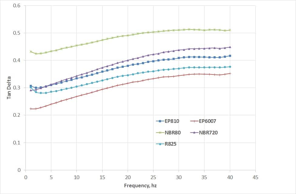
ASTM D5992 covers the methods and process available for determining the dynamic prop- erties of vulcanized natural rubber and synthetic rubber compounds and components. The standard covers the sample shape and size requirements, the test methods, and the pro- cedures to generate the test results data and carry out further subsequent analysis. The methods described are primarily useful over the range of temperatures from cryogenic to 200◦C and for frequencies from 0.01 to 100 Hz, as not all instruments and methods will accommodate the entire ranges possible for material behavior.
Figures(.43and.44) show the results from a frequency sweep test on five (5) different elastomer compounds. Results of Storage modulus and Tan delta are plotted.
Figure .43: Plot of Storage Modulus Vs Frequency from a Frequency Sweep Test
The frequency sweep tests have been carried out by applying a pre-compression of 10 % and subsequently a displacement amplitude of 1 % has been applied in the positive and negative directions. Apart from tests on cylindrical and square block samples ASTM D5992 recommends the dual lap shear test specimen in rectangular, square and cylindri- cal shape specimens. Figure (.45) shows the double lap shear shapes recommended in the standard.
Figure .44: Plot of Tan delta Vs Frequency from a Frequency Sweep Test
Dynamic Properties of Polymer Materials and their Measurements
Polymer materials in their basic form exhibit a range of characteristics and behavior from elastic solid to a viscous liquid. These behavior and properties depend on the temperature, frequency and time scale at which the material or the engineering component is analyzed.
The viscous liquid polymer is defined as by having no definite shape and flow deformation under the effect of applied load is irreversible. Elastic materials such as steels and aluminium deform instantaneously under the application of load and return to the original
state upon the removal of load, provided the applied load is within the yield or plastic limits of the material. An elastic solid polymer is characterized by having a definite shape that deforms under external forces, storing this deformation energy and giving it back upon
the removal of applied load. Material behavior which combines both viscous liquid and solid like features is termed as Viscoelasticity. These viscoelastic materials exhibit a time dependent behavior where the applied load does not cause an instantaneous deformation,
but there is a time lag between the application of load and the resulting deformation. We also observe that in polymeric materials the resultant deformation also depends upon the speed of the applied load.
Characterization of dynamic properties play an important part in comparing mechanical properties of different polymers for quality, failure analysis and new material qualification. Figures 1.4 and 1.5 show the responses of purely elastic, purely viscous and of a viscoelastic material. In the case of purely elastic, the stress and the strain (force and resultant deformation) are in perfect sync with each other, resulting in a phase angle of 0. For a purely viscous response the input and resultant deformation are out of phase by 90o. For a
viscoleastic material the phase angle lies between 0 and 90 degree. Generally the measurements of viscoelastic materials are represented as a complex modulus E* to capture both viscous and elastic behavior of the material. The stress is the sum of an in-phase response and out-of-phase responses.
The so x Cosdelta term is in phase with the strain, while the term so x Sindelta is out of phase with the applied strain. The modulus E’ is in phase with strain while, E” is out of phase with the strain. The E’ is termed as storage modulus, and E” is termed as the loss modulus.
E’ = s0 x cosdelta
E” = s0 x sindelta