Introduction: Advanced Scientific and Engineering Services (AdvanSES), a leading materials science and engineering company, offers advanced testing services to ensure the hyperelasticity of materials used in various applications. From medical devices to aerospace and automotive components, the ability to withstand large deformations without breaking is crucial for their performance and safety. In this blog post, we will delve into the world of hyperelastic material testing at Advanses and explore the techniques and equipment used to evaluate the elastic properties of materials.
Advanses’ Hyperelastic Material Testing Services:
Advanses offers a wide range of testing services to assess the hyperelasticity of materials, including:
Uniaxial Testing: This is the most common type of material testing, where the material is subjected to uniaxial loading in one direction. Advanses uses advanced testing equipment, such as Instron or Zwick, to measure the material’s elastic properties under different loadings.
Multiaxial Testing: This test evaluates the material’s behavior under multidirectional loading conditions, mimicking real-world applications where materials are subjected to multiple forces simultaneously. Advanses’ testing equipment can simulate a variety of loading conditions, including torsion, bending, and compression.
Cyclic Testing: Hyperelastic materials often experience cyclic loading and unloading, which can affect their mechanical properties. Advanses offers cyclic testing services to study the material’s behavior under these conditions and ensure its durability over time.
Dynamic Testing: This test simulates the rapid deformation of materials under dynamic loading conditions, such as those encountered in impact or vibration applications. Advanses’ advanced testing equipment can measure the material’s response to high-speed loading conditions.
Equipment and Techniques Used at Advanses:
Advanses utilizes state-of-the-art equipment and techniques to evaluate the hyperelasticity of materials. Their testing capabilities include:
Universal Testing Machines: These machines are capable of applying forces up to 500,000 Newtons and can simulate a wide range of loading conditions.
Biaxial Testing Machine: This machine is designed for biaxial testing of hyperelastic materials in the aerospace and automotive industries.
Low Velocity Dynamic Testing System: This system enables the measurement of material response at impact speeds, typically in the range of 10s of meters per second. It is useful for evaluating the hyperelasticity of materials under impact loading conditions.
Finite Element Analysis Software: Advanses uses advanced finite element analysis software to simulate the behavior of materials under different loading conditions. This allows them to evaluate the material’s elastic properties without conducting expensive and time-consuming physical tests.
Benefits of Hyperelastic Material Testing at Advanses: By investing in hyperelastic material testing services, companies can gain valuable insights into their materials’ behavior under different loading conditions. The benefits of working with Advanses include:
Improved Material Performance: By understanding the elastic properties of their materials, companies can optimize their design and manufacturing processes to improve performance and safety.
Reduced R&D Costs: Finite element analysis software can significantly reduce the number of physical tests required, saving time and resources in the development process.
Faster Time-to-Market: Advanses’ testing services help companies quickly identify any issues or concerns with their materials, allowing them to address these problems more efficiently and bring their products to market faster.
Enhanced Compliance: By ensuring that their materials meet the required hyperelasticity standards, companies can demonstrate compliance with industry regulations and safety guidelines, reducing the risk of costly recalls or legal action.
Conclusion: Advanses’ hyperelastic material testing services provide companies with valuable insights into their materials’ behavior under different loading conditions. By leveraging their advanced equipment and techniques, businesses can optimize their designs, reduce R&D costs, and ensure compliance with industry regulations. With the ever-increasing demand for innovative materials in various applications, investing in hyperelastic material testing is crucial for companies to stay ahead of the competition and deliver safe and effective products to their customers.
The world of design engineering and materials testing is being reshaped by the advent of artificial intelligence (AI), particularly large language models (LLMs) like Google Bard or ChatGPT. These AI models are not just about generating text; they hold transformative potential for mechanical and materials engineers, especially in the drone and UAV industry.
AI in Design Engineering
LLMs can analyze, interpret, and even generate complex engineering documentation and instructions. This capability allows design and FEA engineers to automate repetitive tasks, freeing them to focus on innovative problem-solving.
These AI models use Natural Language Processing (NLP) techniques to understand codes, clauses, formulas, and standards. With proper fine-tuning, they can develop accurate relationships between engineering variables and requirements within their neural networks. This allows design engineers to create systems that can automatically perform calculations based on the relevant formulas and clauses required for drone design.
AI as a Design Assistant and FEA Engineer
AI can act as a design assistant, capable of making informed decisions and applying codified standards to repetitive types of work. This significantly enhances productivity and efficiency in design engineering workflows.
AI can rapidly generate numerous potential solutions given a problem statement or a design specification. This broadens the design space, uncovering innovative approaches.
AI can also automate many tedious engineering process tasks. For instance, creating CAD models for structure design and analysis can be time-consuming and require a high level of knowledge. However, design engineers can leverage LLMs to instantly generate a CAD model by inputting fundamental design parameters. The LLM can further refine the design based on additional feedback and input provided by the engineer, streamlining the iterative design process.
AI can also play a significant role in material testing. The vast amounts of data that LLMs are trained on means that they can identify patterns and relationships that are not immediately apparent to human designers. Through this unique capability, AI could suggest a material or configuration that increases efficiency or has superior performance compared to more conventional human-led designs.
By leveraging AI’s ability to uncover hidden insights within complex data sets, design engineers can explore novel design possibilities that push the boundaries of conventional engineering practices. This leads to innovative solutions that may have otherwise been overlooked.
Conclusion
The integration of AI into design engineering and materials testing holds significant potential. From automating tedious tasks to generating innovative solutions, AI can act as a powerful tool for design engineers. As we continue to fine-tune these models and explore their capabilities, we can expect to see even more transformative changes in the field of design engineering.
However, it’s important to remember that while AI can enhance and streamline many aspects of design engineering, it doesn’t replace the need for human oversight, intuition, and expertise. The goal is to create a collaborative environment where AI and humans work together, leveraging their respective strengths to drive innovation and efficiency.
So, whether you’re a mechanical materials engineer or a scientist looking to streamline your workflows or a company seeking to stay at the forefront of technological advancements, now is the time to explore the potential of AI and LLMs in your operations. The future of product engineering is here, and it’s powered by AI. At AdvanSES we have already started allocating resources to this emerging field.
Artificial Intelligence (AI) has found numerous applications in mechanical engineering and materials testing, revolutionizing the field with its ability to analyze vast amounts of data and reveal complex interrelationships. Here are some notable applications:
Machine Vision and Learning: AI, particularly machine vision and machine learning, can significantly improve the technical level of material testing¹. Machine vision inputs the characteristics of the inspected object into the computer, while machine learning enables the computer to better analyze these characteristics and make testing conclusions. This process is characterized by high accuracy and speed, and can be used in all aspects of material testing¹.
Textile Material Testing: AI techniques such as image analysis, back propagation, and neural networking can be specifically used as testing techniques in textile material testing. AI can automate processes in various circumstances.
Materials Modeling and Design: AI techniques such as machine learning and deep learning show great advantages and potential for predicting important mechanical properties of materials. They reveal how changes in certain principal parameters affect the overall behavior of engineering materials. This can significantly help to improve the design and optimize the properties of future advanced engineering materials.
Mechanical Engineering: AI, especially machine learning (ML) and deep learning (DL) algorithms, is becoming an important tool in the fields of materials and mechanical engineering. It can predict materials properties, design and development of new materials, and discover new mechanisms of material formation and degradation.
These Artificial Intelligence AI applications in mechanical engineering and materials testing not only enhance the efficiency and accuracy of the testing process but also open up new possibilities for material discovery and design. AdvanSES has decided to be on the forefront of this emerging technology and has invested resources into new developments.
Source: (1) Application of Artificial Intelligence in Material Testing – ResearchGate. https://www.researchgate.net/publication/361295451_Application_of_Artificial_Intelligence_in_Material_Testing/fulltext/637efc6d2f4bca7fd0883bd8/Application-of-Artificial-Intelligence-in-Material-Testing.pdf. (2) Artificial intelligence (AI) in textile industry operational …. https://www.emerald.com/insight/content/doi/10.1108/RJTA-04-2021-0046/full/html. (3) Artificial Intelligence in Materials Modeling and Design. https://link.springer.com/article/10.1007/s11831-020-09506-1. (4) Artificial intelligence and machine learning in design of mechanical …. https://pubs.rsc.org/en/content/articlelanding/2021/mh/d0mh01451f. (5) Evolution of artificial intelligence for application in contemporary …. https://link.springer.com/article/10.1557/s43579-023-00433-3.
Material Characterization Testing of Drones and UAV Materials at AdvanSES
Composite Material Testing for Drones and UAV Applications
Unmanned Aerial Vehicles (UAVs), commonly known as drones, have revolutionized numerous industries, from agriculture and real estate to cinematography and defense. One of the key factors contributing to the versatility and performance of these drones is the use of composite materials in their construction [1,2]. Composite material testing for drones and UAV applications is both difficult and challenging. The use of fiber-reinforced plastic composite materials challenges drone UAV engineers to design and manufacture products with high strength, stiffness and low cost. The demand for more maneuverable, payload effective UAVs is increasing, where composite materials are playing an essential role in the progress of these new high-performance UAV aircrafts with special composite material characteristics like light weight and high strength. These composite materials are distinguished by Young’s modulus as compared to different kinds of metals and aluminum alloys. Multi-rotor type UAVs represent an extremely complex system in terms of design and control. Octacopter, hexacopter and Quadcopter are typical of such multi-rotor designs. Such a type of aircraft is an inherently unstable system, which results from the fact that it cannot independently return to the point of balance (hover) if it loses the functionality of the control loops but will fall or begin to move uncontrollably in space. Furthermore, multirotor UAVs are nonlinear systems since rotor aerodynamic forces and moment characteristics are nonlinear functions with respect to angular velocities and these reasons make the materials used in the manufacturing to be of high quality, load capacity with an infinite fatigue life for the application designed for.
Why Composite Materials?
Composite Material Layered Construction
Composite materials, such as polymers reinforced with carbon fibers (CFRP) and fiberglass (GFRP), are widely used in the manufacturing of drone components, including the fuselage, wings, and landing gear[1].
Polymer composite materials are widely used in various industries, including the manufacturing of drone UAV components, due to their numerous advantages:
High Strength-to-Weight Ratio: Polymer composites, such as those reinforced with carbon or glass fibers, offer a high strength-to-weight ratio[4]. This property is crucial in applications like drone manufacturing, where reducing weight while maintaining strength can enhance performance[4].
Durability: Composites are known for their durability. They do not rust, have high dimensional stability, and can maintain their shape in various conditions. This makes them suitable for outdoor structures and components that are designed to last for a long time.
Design Flexibility: Composites open up new design options that might be hard to achieve with traditional materials. They allow for part consolidation, and their surface texture can be altered to mimic any finish.
Improved Production: With advancements in manufacturing processes, composites are now easier to produce. Digital Composite Manufacturing (DCM), for instance, has made it possible to fabricate composite parts without manual labor.
Material Stability and Insulation: Polymers used in composites offer high material stability against corrosion, good electrical and thermal insulation, and are easy to shape, making them ideal for economic mass production[4].
These advantages make polymer composites an excellent choice for various applications, including the construction of drone components. However, it’s important to note that the use of these materials also necessitates comprehensive testing to ensure safety, reliability, and durability.
Moreover, compared to traditional materials like aluminum, composites can reduce weight by 15-45%, increase corrosion, fatigue, and impact resistance, and reduce noise and vibrations[1].
Testing Composite Materials
Testing composite materials is a critical aspect of ensuring their performance and reliability in various applications, including drone components. Here are some of the common methods used for testing composite materials:
Mechanical Testing: This includes tensile (tension), flexural, impact, shear, and compression testing[1,2]. These tests help determine the material’s strength and deformation under different types of loads.
Physical Testing: This involves tests like water absorption, density, hardness. These tests provide insights into the material’s physical properties and how they might change in different environments.
Thermal Testing: Dynamic Mechanical Analysis (DMA), and Thermomechanical Analysis (TMA) are used to study the material’s thermal properties2.
Moisture Testing: This includes tests like water absorption and moisture conditioning. These tests are crucial for applications where the material might be exposed to moisture.
Analytical Testing: This includes tests like density of core materials, ignition loss, void content, content analysis, and Fourier Transform Infrared Spectroscopy (FTIR). These tests provide a deeper understanding of the material’s composition and structure.
These tests help manufacturers understand the properties of the composite materials that go into a finished product. Composite material testing for drones and UAV applications is both difficult and challenging. The data derived from these tests can be used to compare the composite materials against conventional materials. It’s important to note that the specific tests used can vary depending on the type of composite material and its intended application
Mechanical Testing & Performance Assessment
Uniaxial Tension Test (Directional) (ASTM D638, ISO 527):
The stress (ζ) in a uniaxial tension testis calculated from;
ζ = Load / Area of the material sample ……………………………………..(1)
The strain(ε) is calculated from; ε = δl (change in length) / l (Initial length) ……………..(2)
The slope of the initial linear portion of the curve (E) is the Young’s modulus and given by; E = (ζ2- ζ1) / (ε2- ε1) ……………………………………..(3)
4 Point Bend Flexure Test (ASTM D6272):
The four-point flexural test provides values for the modulus of elasticity in bending, flexural stress, flexural. This test is very similar to the three-point bending flexural test. The major difference being that with the addition of a fourth nose for load application the portion of the beam between the two loading points is put under maximum stress. In the 3 point bend test only the portion of beam under the loading nose is under stress.
4 Point Bend Flexure Test
This arrangement helps when testing high stiffness materials like ceramics infused polymers, where the number and severity of flaws under maximum stress is directly related to the flexural strength and crack initiation in the material. Compared to the three-point bending flexural test, there are no shear forces in the four-point bending flexural test in the area between the two loading pins.
Poisson’s Ratio Test as per ASTM D3039:
Poisson’s ratio is one of the most important parameter used for structure design where all dimensional changes resulting from application of force need to be taken into account, specially for 3d printed materials. For this test method, Poisson’s ratio is obtained from strains resulting from uniaxial stress only. ASTM D3039 is primarily used to evaluate the Poison’s ratio. Testing is performed by applying a tensile force to a specimen and measuring various properties of the specimen under stress. Two strain gauges are bonded to the specimen at 0 and 90 degrees to measure the lateral and linear strains. The ratio of the lateral and linear strain provides us with the Poisson’s ratio.
Flatwise Compression Test as per ASTM D695:
The compressive properties of 3d printed materials are important when the product performs under compressive loading conditions. The testing is carried out in the direction normal to the plane of facings as the core would be placed in a structural sandwich construction. The test procedures pertain to compression call for test conditions where the deformation is applied under quasi-static conditions negating the mass and inertia effects.
Uniaxial Flatwise Compression Testing
The test procedures pertaining to compression call for test conditions where the deformation is applied under quasi-static conditions negating the mass and inertia effects.
Modified Compression Test as per Boeing BSS 7260:
Modified ASTM D695 and Boeing BSS 7260 is the testing specification that determines compressive strength and stiffness of polymer matrix composite materials using a loading compression test fixture. This test procedure introduces the compressive force into the specimen through end loading.
Modified Compression Test as per Boeing BSS 7260
Axial Fatigue Test as per ASTM D7791 & D3479:
ASTM D7791 describes the determination of dynamic fatigueproperties of plastics in uniaxial loading conditions. Rigid or semi-rigid plastic samples are loaded intension (Procedure A) and rigid plastic samples are loaded incompression (Procedure B) to determine the effect of processing, surface condition, stress, and such,on the fatigue resistance of plastic and reinforced composite materials subjected to uniaxial stress for a large number of cycles.The results are suitable for study of high load carrying capability of candidate materials. ASTM recommends a test frequency of 5hz or lower.The tests can be carried out under load/stress or displacement/strain control. The test method allows generation of stress or strain as a function of cycles, with the fatigue limit characterized by failure of the specimen or reaching 10E+07 cycles.The maximum and minimum stress or strain levels are defined throughan R ratio.
Axial Fatigue Test as per ASTM D7791
3 Point Bend Flexure Test (ASTM D790):
Three point bending testing is carried out to understand the bending stress, flexural stress and strain of composite and thermoplastic 3d printed materials. The specimen is loaded in a horizontal position, and in such a way that the compressive stress occurs in the upper portion and the tensile stress occurs in the lower portion of the cross section.This is done by having round bars or curved surfaces supporting the specimen from underneath. Round bars or supports with suitable radii are provided so as to have a single point or line of contact with the specimen. The load is applied by the rounded nose on the top surface of the specimen. If the specimen is symmetrical about its cross section the maximum tensile and compressive stresses will be equal. This test fixture and geometry provides loading conditions so that specimen fails in tension or compression.
3 Point Bend Flexure Test
For most composite materials,the compressive strength islower than the tensile and thespecimen will fail at thecompression surface. This compressive failure isassociated with the localbuckling (micro buckling) ofindividual fibres.
Drop Weight low Velocity Impact Test (ASTM D7136, ISO 6603):
The importance of understanding the response of structural composites to impact events cannot be emphasized enough. Low velocity impact occurs at velocities below 10 m/s and is likely to cause some dents and visible damage on the surface due to matrix cracking and fibre breaking, as well as delamination of the material. In some materials, impact tests characterize the face sheet quality and if they are suitable for the application.
Drop Weight low Velocity Impact Test
Summary:
A variety of standardized mechanical tests on unreinforced and reinforced 3d printed materials including tension, compression, flexural,and fatigue have been discussed.
Mechanical properties of 3d printed polymers, fiber-reinforced polymeric composites immensely depend on thenature of the polymer filament, fiber, and the layer by layer interfacial bonding. Advanced engineering design and analysis applications like Finite Element Analysis use this mechanical test data to characterize the materials. These material properties can be used to develop material models for use in FEA softwares like Ansys, Abaqus, LS-Dyna, MSC-Marc etc.
Conclusion
The use of composite materials in drone manufacturing presents a promising avenue for enhancing UAV performance. However, it also necessitates comprehensive testing to ensure the safety, reliability, and durability of these drones. As the drone industry continues to grow and evolve, so too will the methods for testing and optimizing the use of composite materials in drone construction.
Keywords: UAV, composite materials, drone components, material testing, CFRP, GFRP, finite element analysis, bending test.
References:
M Sönmez, Ce Pelin, M Georgescu, G Pelin, Md Stelescu, M Nituica, G Stoian, Unmanned Aerial Vehicles – Classification, Types Of Composite Materials Used In Their Structure And Applications.
Camil, Lancea et al., Simulation, Fabrication and Testing of UAV Composite Landing Gear. MDPI Journal, https://doi.org/10.3390/app12178598
National Research Council, Airframe Materials and Structures, Enabling Science for Military Systems
Non-linear Hyperelastic Material Characterization Testing for FEA
The characterization of materials for Finite Element Analysis (FEA) and Computational Fluid Dynamics (CFD) is a specialized process that involves extensive laboratory testing. At AdvanSES, we have become industry leaders in this field, particularly with our focus on the characterization of polymer materials. Through a series of specific tests, we are able to determine the unique properties of each material, thus providing valuable data for FEA and CFD.
Pure Shear
Our testing process begins with a pure shear test. This involves applying uniaxial tension to a test specimen using either a parallel or tangential method. The response of the material to this stress provides a baseline understanding of its characteristics under tension.
Volumetric Compression
We then proceed to a volumetric compression test. This study involves placing a sample of the material under hydrostatic compression deformation. The way the material responds to this form of stress provides valuable data on its behavior under compression.
Uniaxial Compression
Uniaxial compression testing is another key component of our testing process. Here, we evaluate the response of the material when compression stress is applied along a single axis. This test gives us a clear picture of how the material behaves under a single axis of compression stress.
Uniaxial Tension
Uniaxial tension testing involves applying tensile stress to a specimen. The result of this test provides us with further insights into the behavior of the material under tension.
Biaxial Tension
A biaxial tension test involves placing tensile stress on a specimen in two simultaneous directions. This test is particularly useful in understanding the behavior of a material under multiple tensions.
Creep and Stress Relaxation
The final testing stage is the creep and stress relaxation test. This involves a uniaxial tensile test followed by the maintenance of the elongation on the specimen for a specified duration. By observing the material’s response over this period, we can gain valuable insights into the long-term behavior of the material under stress.
Our laboratory is located at Plot No. 49, Mother Industrial Park, Zak-Kadadara Road, Kadadara, Taluka: Dehgam, District: Gandhinagar, Gujarat 382305, India.
For more information about our services and how we can assist with your material characterization needs, give us a call at +91-9624447567 or send us an email at [email protected].
Installation of mechanical testing structural load frame for carrying out testing high capacity load bearing components. Frames are now available for comprehensive engineering validation of automotive, railways, aerospace components and structures made from polymers, metallic and composite materials.
We can now test and break products and materials from 5N to 500KN.
At AdvanSES, we provide a full 360 degree static and dynamic characterization of your materials, parts and components. We measure the tension, compression, shear, vibration and dynamic properties of individual components and sub assemblies in accordance to international standards.
Plastic Material Testing: Ensuring Quality and Safety
Plastic materials have become an integral part of our lives, from the packaging of our daily essentials to the construction of our homes and buildings. However, the use of plastics has also raised concerns about their impact on the environment and human health. Therefore, it is essential to test plastic materials to ensure their quality and safety. At AdvanSES plastic material testing is carried out under the strict and rigorous quality control as per ISO 17025:2017 testing conditions.
Plastic material testing involves analyzing the physical, chemical, and mechanical properties of plastic materials. These tests provide valuable information about the durability, strength, and chemical resistance of plastics, which are critical factors in determining their suitability for specific applications.
Types of Plastic Material Testing
Fatigue Testing at AdvanSES
There are various types of plastic material testing, each serving a specific purpose. The most common types of tests include:
Tensile Testing: This test measures the strength of plastic materials under tension, providing valuable information about their mechanical properties.
Impact Testing: This test evaluates the ability of plastic materials to withstand sudden impact, which is critical in applications such as packaging and transportation.
Fatigue Testing: This test evaluates the ability of plastic materials to withstand long term service loads, the mechanical service life of the materials and parts can be predicted from fatigue testing.
Thermal Analysis: This test measures the thermal properties of plastic materials, such as their melting and crystallization behavior.
Chemical Resistance Testing: This test evaluates the resistance of plastic materials to various chemicals, providing important information about their suitability for use in specific environments.
Flammability Testing: This test evaluates the ability of plastic materials to resist ignition and combustion, providing critical information for applications such as building construction.
At AdvanSES, we provide plastic and composite material testing under all the above mentioned parameters, you can be worry free about our test data and results as we are ISO 17025:2017 accredited.
Benefits of Plastic Material Testing
Plastic material testing offers numerous benefits, including:
Quality Control: Plastic material testing helps to ensure that plastic materials meet quality standards, reducing the risk of product failure and liability.
Cost Savings: By identifying potential defects or weaknesses in plastic materials early on, testing can help to reduce production costs and minimize waste.
Safety: Plastic material testing ensures that plastic materials are safe for use in specific applications, protecting both consumers and the environment.
We can provide a quick quote for your plastic and composite material testing needs within a business day, try giving us a call or email and we would be happy to assist with any of your testing needs.
Conclusion
Plastic material testing plays a critical role in ensuring the quality and safety of plastic materials. By analyzing their physical, chemical, and mechanical properties, testing provides valuable information about their suitability for specific applications. By optimizing this blog post for search engines, we can ensure that this important information reaches a wider audience, promoting greater awareness of the importance of plastic material testing.
Do you know the critical tearing energy of your rubber material?
Critical tearing energy is an important parameter to study crack growth in rubber under fatigue loading and it’s evaluation becomes imperative for the design and evaluation of rubber products. To prevent crack growth and sudden fatigue failures, one of the technique is to improve the tearing energy of rubber. Evaluation and testing of tearing energy properties is of utmost importance.
In automotive, aerospace and biomedical applications, soft elastomers and rubbers often handle cyclic loads and displacement cycles during their entire service duty cycle. When going through long periods of cyclic loading, catastrophic failure frequently happens becuase of crack formation, growth followed by propagation.
Contact us to evaluate the critical energy of your rubber material. More information at https://www.advanses.com
Join our mailing list and stay up to date on related resources and discussions. We carry out standardized as well as custom testing.
A proper treatment of the rubber material testing service conditions and material degradation phenomena like strain softening is of prime importance in the testing of rubbers specimens for FEA material characterization. The accuracy and reliability of obtained test data depends on how the mechanical conditioning and representational service conditions of the material have been accounted for in the test data. To simulate a component in unused and unaged conditions, the mechanical conditioning requirements are different than the ones for simulating a component that has gone through extensive field service and aging under different environmental conditions.
To simulate performance of a material or component by Finite Element Analysis (FEA) it should be tested under the same deformation modes to which original assembly will be subjected. The uniaxial tension tests are easy to perform and are fairly well understood but if the component assembly experiences complex multiaxial stress states then it becomes imperative to test in other deformation modes. Planar (pure shear), biaxial and volumetric (hydrostatic) tests need to be performed along with uniaxial tension test to incorporate the effects of multiaxial stress states in the FEA model.
Material stiffness degradation phenomena like Mullin’s effect at high strains and Payne’s effect at low strains significantly affect the stiffness properties of rubbers. After the first cycle of applied strain and recovery the material softens, upon subsequent stretching the stiffness is lower for the same applied strain.
Despite all the history in testing hyperelastic and viscoelastic materials, there is a lack of a methodical and standard testing protocol for pre-conditioning. Comprehensive studies on the influence of pre-conditioning are not available. Readers are referred to Austrell[] and Remache, et al,[]. There are no guidelines for sample pre-conditioning in ASTM D412. However, British Standard BS 903 suggests to perform 5 cycles of pre-conditioning to improve test reproducibility.
There are five (5) different techniques to carry out pre-conditioning and material testing of general elastomer samples.
1. The first technique pertains to a mechanical test where the the testing of the sample is carried out under one single stretch at a speed recommended by the ASTM D412 specification.
2. In the second testing technique the sample is stretched at a constant speed up to the maximum relevant strain brought back to the initial position. Cyclic stretching is then carried out for anywhere for 1 to 7 cycles. The speed of the initial stretch and the number of subsequent cyclic stretches needs to be same. The data curve is then shifted to the origin by zeroing out the stress and strain and used for curve-fitting procedure.
3. In the third testing protocol the sample is stretched to a fraction of the full material stretch capability and brought back to the initial position and cycled back again to this fractional position anywhere from 2 to 7 cycles. The stretch in the sample is then increased to the second level and cycled back to initial position multiple times. The sample is stretched back to an even higher position and cycled back. This progressively continues until the maximum strain capability of the material is reached. This protocol is known as progressive pre-conditioning.
4. In the fourth testing technique the sample is stretched to a fraction of the total stretch capability and relaxed for anywhere from 30 seconds to 120 seconds as per the material. The sample is then again stretched to a higher limit and relaxed again. This is continued until the maximum stretchable capability of the material. This particular technique stretches the material and allows the material to fully creep and relax at each interval so that all the stress softening is accounted for in the test data.
5. In the fifth testing technique the sample is tested under a single stretch but the speed or the rate of stretch is very slow. This ultra-slow speed test is carried out so that the material can creep, relax, and the cross-links in the elastomer are given enough time to expand-contract and come to a balanced position during the stretching. This technique is a combination of the two above testing techniques.
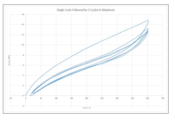
These five (5) testing protocols involve the stretching of the material to different limits under different conditions and suitably cycling the material. The suitability of one testing technique over the other is debatable and one should adopt the technique that most closely resembles the operating conditions of the material and what one expects to back out from the Finite Element Analysis. Figures (1.11) through (1.14) shows the results from using the different testing protocols on a 55 durometer Natural Rubber Compound that finds general application in an automotive engine mount.
Figure 1.11: Uniaxial Tension Test Results
Figure 1.12: Single Stretch Followed by 3 Cycles of Stretching to the Maximum
Figure (1.12) shows the results from comparisons carried out on a uniaxial compression test for an engine mount material characterization. Two protocols were employed to carry out the material characterization. Progressive straining and cycling was carried out first. The material was strained 3 times before reaching the ultimate strain of approximately 75 %. The material was subsequently tested using ultra slow straining protocol. As can be seen the test data output for FEA input is the same using both the techniques. This result confirms the observation by Austrell in his work on conditioning of material samples for characterization i.e., Mullins effect can be negated when enough time is allowed for the material to relax, creep, and flow during the rubber material testing.
Figure 1.13: Progressive Pre-conditioning with Stretching to 3 levels and Cyclic Stretches
Figure 1.14: Progressive Relaxation, Stretching and Relaxation to Maximum Levels
1.2 Guidelines for Rubber Material Testing
Rubber compounds are formulated from recipes of ingredient materials. Depending on the time, location and environment while mixing the compounds, properties are known to vary from batch to batch.
• All testing to characterize a material compound should be performed on the same batch.
• Laboratory validations will help to correlate test specimen slabs against the real components to make sure they have identical cure history.
• Small compression buttons can be extracted from components and compared with slab data.
• The testing should be carried out at the temperature at which the component is expected to perform under field service conditions.
• For seals and o-rings, aging in oils and solutions can be carried out prior to testing.
• Input of more than one test data type in FEA software will increase simulation accuracy by an order of magnitude
We at AdvanSES are capable of developing a custom testing protocol for compliance with international standards or for quality assurance. Materials testing services offered by AdvanSES include:
Composition: Whe you need to know with certainty what materials are used in the manufacture of thermoplastics, rubber materials etc.
Shear Test: Materials testing designed to measure shear strength of rubber and composites. These tests show how much stress a specimen can take before failure and is often times used to test and compare the strength of adhesives.
Flexural Test: When a product like an I-beam or girder used in construction must support a predetermined amount of weight without sagging, a flexure materials test is often performed to verify that the specimen can withstand a certain level of stress without flexing.
Environment and High Temperature Exposure Test: When it comes to determining the lifespan of materials, especially elastomer materials intended for outdoor use, exposure to high temperature and oils is carried out to check the degradation of materials.
Tensile/Compression Tests: From plastics and metals to adhesives and rubbers, tensile/compression testing is a form of materials testing that places specimens under precise compressive loads to measure their ability to withstand compression before deformation occurs.
Fatigue Tests: Fatigue tests are important to determine the endurance or breaking load a material can withstand before failing as well as the number of repeated loading cycles it can endure. Fatigue testing looks at a materials limit to withstand stresses and environment degradation. We can conduct stress controlled and strain controlled high cycle fatigue tests from room temperature to 250C on material samples, parts and components.
Applications of Materials Testing:
1) Quality Control 2) Regulatory Compliance 3) Design Development 4) Failure Analysis 5) Performance Prediction 6) Finite Element Analysis Material Constants Data