Rubber FEA & Hyperelastic Characterization of Elastomers and Rubber Materials
Hyperelastic Material Modeling using Ansys, Abaqus, Marc in Finite element analysis (FEA) software packages is widely used in the design and analysis of polymeric rubber and elastomer components in the automotive and aerospace industry. Test data from the major principal deformation modes are used to develop the hyperelastic material constants to account for the different states of strain.
Uniaxial tension is the mother of all mechanical tests and provides a very important data point regarding the strength, toughness and quality of the material. ASTM and ISO standards provide the guidance to carry out the tests. The samples are designed so as the specimen length is larger than the width and thickness. This provides a uniform tensile strain state in the specimen.
2) Planar Shear Testing
Planar shear specimens are designed so that the width is much larger than the thickness and the height. Assuming that the material is fully incompressible the pure shear state exists in the specimen at a 45 degree angle to the stretch direction.
3) Volumetric Compression Testing
The measure of compressibility of the material is testing using the Volumetric compression test. A button specimen is used and a hydrostatic state of compression is applied on the specimen to evaluate it.
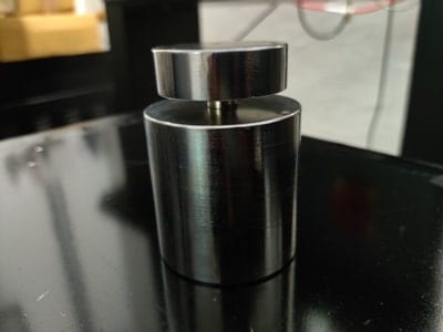
4) Uniaxial Compression Testing
Uniaxial compression refers to the compression of a button specimen of approx. 29mm diameter and 12.5 mm height. This test can be effectively utilized to replace the expensive biaxial extension test through proper control of the specimen and testing fixture surface friction and proper testing technique and methodology.
5) EquiBiaxial Tension Testing
Biaxial tensile testing is a highly accurate testing technique for mechanical characterization of soft materials. Typical materials tested in biaxial tension are soft and hard rubbers elastomers, polymeric thin films, and biological soft tissues.
The outputs from these tests are the stress vs strain curves in the principal deformation modes. Curve fitting is carried out on the experimental stress vs strain curves to generate the material constants.
These constants are obtained by comparing the stress- strain results obtained from the material model to the stress-strain data from experimental tests. Iterative procedure using least-squares fit method is used to obtain the constants, which reduces the relative error between the predicted and experimental values. The linear least squares fit method is used for material models that are linear in their coefficients e.g Neo-Hookean, Mooney-Rivlin, Yeoh etc. For material models that are nonlinear in the co-efficient relations e.g. Ogden etc, a nonlinear least squares method is used.
Errors and uncertainties in the application of FEA for Composite Materials can come from the following many sources,
1) Errors that come from the inherent assumptions in the FEA theory and
2) Errors and uncertainties that get built into the system when the physics we are seeking to model gets transferred to FEA models.
A common list of these kind of errors are as mentioned below;
> Errors and uncertainties from the solver. > Level of mesh refinement and the choice of element type. > Averaging and calculation of stresses and strains from the primary solution variables. > Approximations in the material properties of the model. > Approx. and uncertainties in the loading and boundary conditions of the model.
The long list of error sources and uncertainties in the procedure makes it desirable that a framework of rules and criteria are developed for the application of finite element method. Verification procedure includes checking the design, the software code and also investigate if the computational model accurately represents the physical system. Validation is more of a dynamic procedure and determines if the computational simulation agrees with the physical phenomenon, it examines the difference between the numerical simulation and the experimental results. Verification provides information whether the computational model is solved correctly and accurately, while validation provides evidence regarding the extent to which the mathematical model accurately correlates to experimental tests.
The blue, red and green colored areas in Figure highlight the iterative validation and verification activities in the process. The green highlighted region falls in the domain of the laboratory performing the experiments.
Comparing the issue of code verification and calculation verification of FEA for Composite Materials, the main point of difference is that calculation verification involves quantifying the discretization error in the simulation. Code verification is rather upstream in the process and is done by comparing numerical results with analytical solutions.
The validation procedure has to be developed by the analyst. The following validation guidelines were developed at Sandia National Labs [Oberkampf et al.] by experimentalists, these are applicable to all problems from computational mechanics.
#1: The validation experiment should be designed by the FEA group & experiment engineers. The experiments should be designed so that validation falls inside the application domain. #2: The designed experiment should involve the full physics of the system, including the loading and boundary conditions. #3: The solutions of the experiments and from the computational model should be totally independent of each other. #4: The experiments and the validation process should start from the system level solution to the component level. #5: Care should be taken that operator bias or process bias does not contaminate the solution or the validation process.
Hyperelastic viscoelastic testing of rocket propellants. Solid propellant is the power source of a solid rocket motor. The mechanical properties of a solid rocket motor directly affect the load carrying capacity of a rocket. AdvanSES can provide multiaxial mechanical property characterization of these solid rocket propellants based on hyperelastic and viscoelastic tests.
AdvanSES’ hyperelastic and viscoelastic material characterization tests for solid rocket propellant materials include;
The sole purpose of an engineering laboratory is to provide engineering product development and problem solving services to industries by carrying out controlled condition experiments and engineering analysis. These controlled condition experiments are done using testing machines, computational mechanics tools and advanced engineering softwares. At AdvanSES we use state of the art testing equipments to conduct material testing on any kind of metals, polymers and composite materials. Our computational mechanics tools like Abaqus Finite element analysis software, our in-house machine shop aid us in this process.
Material Testing:
Testing methodologies are primarily divided into two (2) categories depending upon the test rate; static and dynamic. AdvanSES has both static and dynamic testing capabilities. We are able to provide a full 360 degree view of any material or product’s mechanical characteristics. We can also strength, strain, fatigue, hardness, and lots more.
Our testing methods include the following:
1. ASTM D638 – Standard Test Method for Tensile Properties of Plastic
2. ASTM D882 – Standard Test Method for Tensile Properties of Thin Plastic Sheeting
3. ASTM D412 – Standard Test Methods for Vulcanized Rubber and Thermoplastic Elastomers in Tension
1) An Independent, design analysis and mechanical testing laboratory. 2) More than 2 decades of product testing and application expertise in mechanical, and materials engineering. 3) State of the art materials and mechanical testing laboratory with qualified engineers. 4) Innovative design, analysis and testing solutions for a wide range of industries
Non-linear Viscoelastic Dynamic Properties of Polymer, Rubber and Elastomer Materials
Static testing of materials as per ASTM D412, ASTM D638, ASTM D624 etc can be categorized as slow speed tests or static tests. The difference between a static test and dynamic test is not only simply based on the speed of the test but also on other test variables em- ployed like forcing functions, displacement amplitudes, and strain cycles. The difference is also in the nature of the information we back out from the tests. When related to poly- mers and elastomers, the information from a conventional test is usually related to quality control aspect of the material or the product, while from dynamic tests we back out data regarding the functional performance of the material and the product.
Tires are subjected to high cyclical deformations when vehicles are running on the road. When exposed to harsh road conditions, the service lifetime of the tires is jeopardized by many factors, such as the wear of the tread, the heat generated by friction, rubber aging, and others. As a result, tires usually have composite layer structures made of carbon-filled rubber, nylon cords, and steel wires, etc. In particular, the composition of rubber at different layers of the tire architecture is optimized to provide different functional properties. The desired functionality of the different tire layers is achieved by the strategical design of specific viscoelastic properties in the different layers. Zones of high loss modulus material will absorb energy differently than zones of low loss modulus. The development of tires utilizing dynamic characterization allows one to develop tires for smoother and safer rides in different weather conditions.
Figure Locations of Different Materials in a Tire Design
The dynamic properties are also related to tire performance like rolling resistance, wet traction, dry traction, winter performance and wear. Evaluation of viscoelastic properties of different layers of the tire by DMA tests is necessary and essential to predict the dynamic performance. The complex modulus and mechanical behavior of the tire are mapped across the cross section of the tire comprising of the different materials. A DMA frequency sweep
test is performed on the tire sample to investigate the effect of the cyclic stress/strain fre- quency on the complex modulus and dynamic modulus of the tire, which represents the viscoelastic properties of the tire rotating at different speeds. Significant work on effects of dynamic properties on tire performance has been carried out by Ed Terrill et al. at Akron Rubber Development Laboratory, Inc.
Non-linear Viscoelastic Tire Simulation Using FEA
Non-linear Viscoelastic tire simulation is carried out using Abaqus to predict the hysteresis losses, temperature distribution and rolling resistance of a tire. The simulation includes several steps like (a) FE tire model generation, (b) Material parameter identification, (c) Material modeling and (d) Tire Rolling Simulation. The energy dissipation and rolling re- sistance are evaluated by using dynamic mechanical properties like storage and loss modu- lus, tan delta etc. The heat dissipation energy is calculated by taking the product of elastic strain energy and the loss tangent of materials. Computation of tire rolling is further carried out. The total energy loss per one tire revolution is calculated by;
Ψdiss = ∑ i2πΨiTanδi, (.27)
i=1
where Ψ is the elastic strain energy,
Ψdiss is the dissipated energy in one full rotation of the tire, and
Tanδi, is the damping coefficient.
The temperature prediction in a rolling tire shown in Fig (2) is calculated from the loss modulus and the strain in the element at that location. With the change in the deformation pattern, the strains are also modified in the algorithm to predict change in the temperature distribution in the different tire regions.
Polymeric rubber components are widely used in automotive, aerospace and biomedical systems in the form of vibration isolators, suspension components, seals, o-rings, gaskets etc. Finite element analysis (FEA) is a common tool used in the design and development of these components and hyperelastic material models are used to describe these polymer materials in the FEA methodology. The quality of the CAE carried out is directly related to the input material property and simulation technology. Nonlinear materials like polymers present a challenge to successfully obtain the required input data and generate the material models for FEA. In this brief article we review the limitations of the hyperleastic material models used in the analysis of polymeric materials.
Theory:
A material model describing the polymer as isotropic and hyperelastic is generally used and a strain energy density function (W) is used to describe the material behavior. The strain energy density functions are mainly derived using statistical mechanics, and continuum mechanics involving invariant and stretch based approaches.
Statistical Mechanics Approach
The statistical mechanics approach is based on the assumption that the elastomeric material is made up of randomly oriented molecular chains. The total end to end length of a chain (r) is given by
Where µ and lm are material constants obtained from the curve-fitting procedure and Jelis the elastic volume ratio.
Invariant Based Continuum Mechanics Approach
The Invariant based continuum mechanics approach is based on the assumption that for a isotropic, hyperelastic material the strain energy density function can be defined in terms of the Invariants. The three different strain invariants can be defined as
I1 = l12+l22+l32
I2 = l12l22+l22l32+l12l32
I3 = l12l22l32
With the assumption of material incompressibility, I3=1, the strain energy function is dependent on I1 and I2 only. The Mooney-Rivlin form can be derived from Equation 3 above as
With C01 = 0 the above equation reduces to the Neo-Hookean form.
Stretch Based Continuum Mechanics Approach
The Stretch based continuum mechanics approach is based on the assumption that the strain energy potential can be expressed as a function of the principal stretches rather than the invariants. The Stretch based Ogden form of the strain energy function is defined as
where µiand αi are material parameters and for an incompressible material Di=0.
Neo-Hookean and Mooney-Rivlin models described above are hyperelastic material models where, the strain energy density function is calculated from the invariants of the left Cauchy-Green deformation tensor, while in the Ogden material model the strain energy density function is calculated from the principal deformation stretch ratios.
The Neo-Hookean model, one of the earliest material model is based on the statistical thermodynamics approach of cross-linked polymer chains and as can be studied is a first order material model. The first order nature of the material model makes it a lower order predictor of high strain values. It is thus generally accepted that Neo-Hookean material model is not able to accurately predict the deformation characteristics at large strains.
The material constants of Mooney-Rivlin material model are directly related to the shear modulus ‘G’ of a polymer and can be expressed as follows:
G = 2(C10+ C01) …………………………….…(6)
Mooney-Rivlin model defined in equation (4) is a 2nd order material model, that makes it a better deformation predictor that the Neo-Hookean material model. The limitations of the Mooney-Rivlin material model makes it usable upto strain levels of about 100-150%.
Ogden model with N=1,2, and 3 constants is the most widely used model for the analysis of suspension components, engine mounts and even in some tire applications. Being of a different formulation that the Neo-Hookean and Mooney-Rivlin models, the Ogden model is also a higher level material models and makes it suitable for strains of upto 400 %. With the third order constants the use of Ogden model make it highly usable for curve-fitting with the full range of the tensile curve with the typical ‘S’ upturn.
Discussion and Conclusions:
The choice of the material model depends heavily on the material and the stretch ratios (strains) to which it will be subjected during its service life. As a rule-of-thumb for small strains of approximately 100 % or l=2.0, simple models such as Mooney-Rivlin are sufficient but for higher strains a higher order material model as the Ogden model may be required to successfully simulate the ”upturn” or strengthening that can occur in some materials at higher strains.
REFERENCES:
ABAQUS Inc., ABAQUS: Theory and Reference Manuals, ABAQUS Inc., RI, 02
Attard, M.M., Finite Strain: Isotropic Hyperelasticity, International Journal of Solids and Structures, 2003
Bathe, K. J., Finite Element Procedures Prentice-Hall, NJ, 96
Bergstrom, J. S., and Boyce, M. C., Mechanical Behavior of Particle Filled Elastomers,Rubber Chemistry and Technology, Vol. 72, 2000
Beatty, M.F., Topics in Finite Elasticity: Hyperelasticity of Rubber, Elastomers and Biological Tissues with Examples, Applied Mechanics Review, Vol. 40, No. 12, 1987
Bischoff, J. E., Arruda, E. M., and Grosh, K., A New Constitutive Model for the Compressibility of Elastomers at Finite Deformations, Rubber Chemistry and Technology,Vol. 74, 2001
Blatz, P. J., Application of Finite Elasticity Theory to the Behavior of Rubber like Materials, Transactions of the Society of Rheology, Vol. 6, 196
Kim, B., et al., A Comparison Among Neo-Hookean Model, Mooney-Rivlin Model, and Ogden Model for Chloroprene Rubber, International Journal of Precision Engineering & Manufacturing, Vol. 13.
Boyce, M. C., and Arruda, E. M., Constitutive Models of Rubber Elasticity: A Review, Rubber Chemistry and Technology, Vol. 73, 2000.
Srinivas, K., Material Characterization and FEA of a Novel Compression Stress Relaxation Method to Evaluate Materials for Sealing Applications, 28th Annual Dayton-Cincinnati Aerospace Science Symposium, March 2003.
Srinivas, K., Material Characterization and Finite Element Analysis (FEA) of High Performance Tires, Internation Rubber Conference at the India Rubber Expo, 2005.